Entrain spatial ligand-velocity analysis (with Visium+scRNA).
entrain_spatial_velocity_output.RmdThis document outlines an Entrain analysis, in Python, starting from
an scverse anndata object with pre-calculated
velocities and a second anndata object containing 10x
Visium data. By the end of this document, you will identify ligands that
are predicted to both:
A. Drive the velocities in your data, and
B. Co-localize with their corresponding receptors.
Prior Assumptions and Caveats
Entrain-Spatial Analysis requires the following:
- A
.h5adobject containing Visium spatial transcriptomics RNA-seq data on a dataset of cells differentiating as well as cells comprising their microenvironmental niche. - A
.h5adobject containing10x Chromiumsingle-cell RNA-seq data that contains cells of similar biology to the Visium.h5ad. Please ensure that your biology you are interested in is conducive to producing trustworthy velocities.. Please also ensure that both.h5adobjects contain data on similar biological phenomena, such as similar cell type proportions.
Other sequencing chemistries: We prefer Visium because it maps the whole-transcriptome and therefore we are confident that the majority of relevant ligand-receptor genes will be present in the raw data. Entrain has not been tested with chemistries involving non-Visium spatial technologies. Hybridization-based technologies may be possible, but please ensure your panel encapsulates enough ligand-receptor genes. A ligand-receptor that is not sequenced by your technology will not be discoverable.
Secreted ligands: Ligands that do not require spatial proximity to be active, such as secreted ligands, will be found only if their corresponding receptor is expressed adjacent to the cell that is expressing the mRNA for that ligand.
Setup
Required python packages for spatial analysis
conda install squidpy scanpy rpy2 scvelo adjusttext r-randomforest matplotlib seaborn scikit-learn
pip install tangram-sc
pip install pypath-omnipath
pip install entrain
Load Data and Visualize
First, download the test data from
https://zenodo.org/record/7874401 into your working
directory and load required packages.
import entrain as en
import anndata as ad
import pandas as pd
import scanpy as sc

velocity_adata_file = "ratz_atlas_velocities_sparse.h5ad"
spatial_adata_file = "v11_vis.h5ad"
ligand_target_matrix_file = "ligand_target_matrix_mm.csv"

adata = ad.read_h5ad(velocity_adata_file)
adata_st = ad.read_h5ad(spatial_adata_file)
ligand_target_matrix = pd.read_csv(ligand_target_matrix_file, index_col=0)
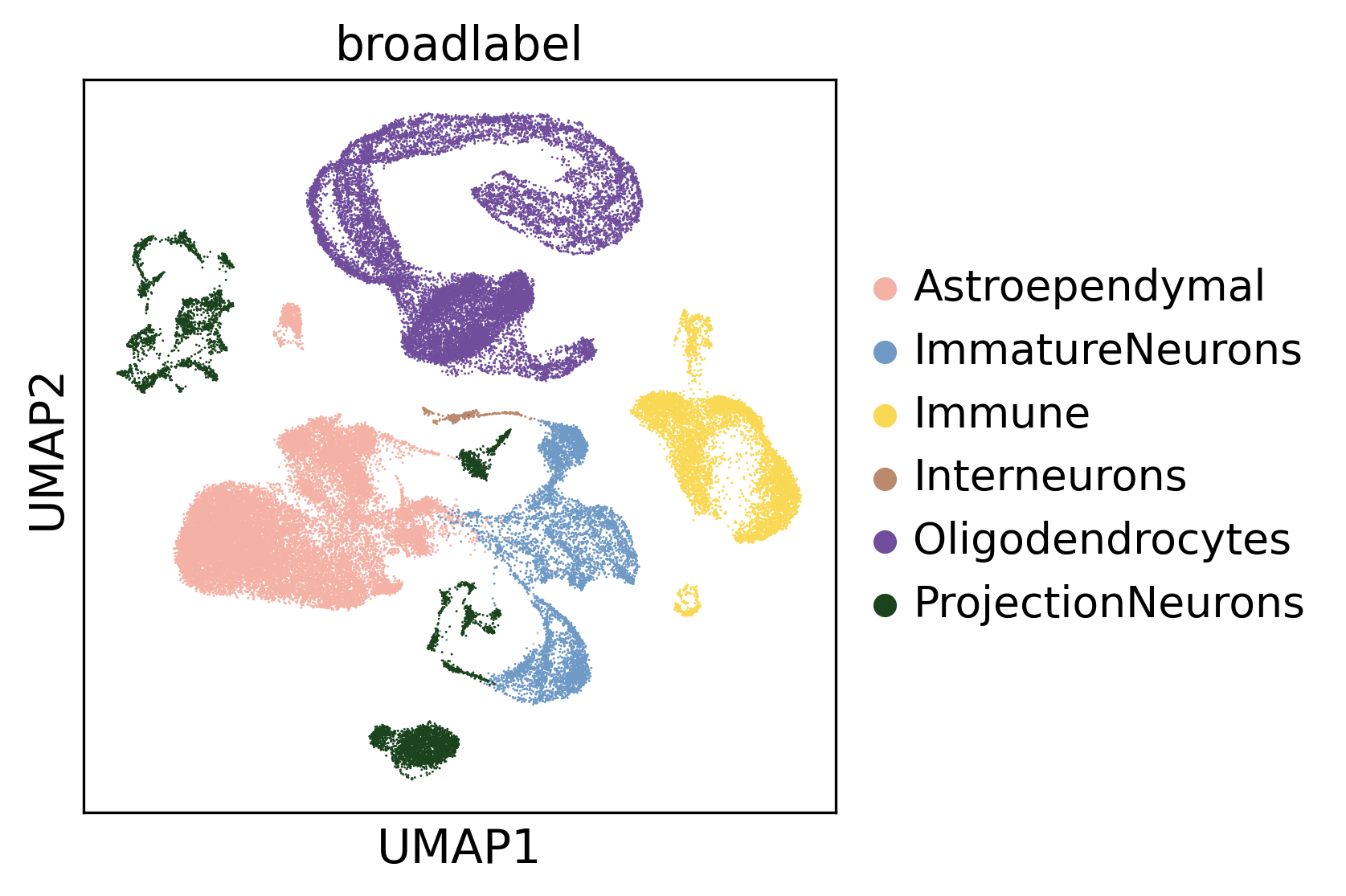
The dataset comprises a population of developing neuronal precursors, astrocytes, oligodendrocytes, and cells of their respective niches.
sc.pl.umap(adata, color = "broadlabel", palette = adata.uns["broad_label_palette"])
Cluster Velocities
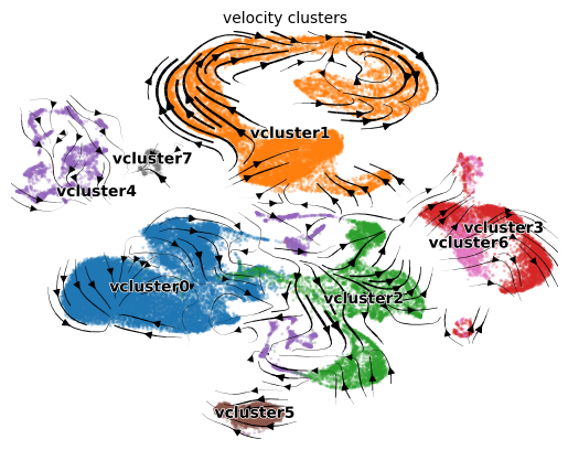
As in the entrain velocity analysis vignette, cluster
our velocities into major differentiation clusters.
adata = en.cluster_velocities(adata)
en.plot_velocity_clusters_python(adata,
                                 plot_file = "plot_velocity_clusters.png",
                                velocity_cluster_key = "velocity_clusters")
Recover Dynamics
Velocity likelihoods for each cluster are then calculated via scvelo, to feed into later Entrain analysis.
adata = en.recover_dynamics_clusters(adata,
                              n_jobs = 10,
                              return_adata = True,
n_top_genes=None)- Note that as of July 2023, there is an existing bug in
scvelo.tl.recover_dynamics(). Using `numpy version 1.23.5 may fix the problem. Also see #1058.
If some of your clusters contain few cells, you may get numerous
warnings
e.g. WARNING: TDRD6 not recoverable due to insufficient samples..
This is expected in clusters that contain few cells. If you’d like to
remove these clusters from further analysis, you can specify the
argument vclusters = in the next step.
Run Spatial Entrain
The following function performs the following steps: 1. Perform label transfer (via tangram) on the velocity clusters to map velocities to their spatial context. 2. Identify ligand-receptor pairs between adjacent Visium spots. 3. Fit a random forest model to the velocity likelihoods to identify ligand signals that are influencing the observed velocities.
adata_result=en.get_velocity_ligands_spatial(adata,
                                             adata_st,
                                             organism="mouse",
                                             velocity_cluster_key = "velocity_clusters",
                                             ligand_target_matrix=ligand_target_matrix)
Visualization
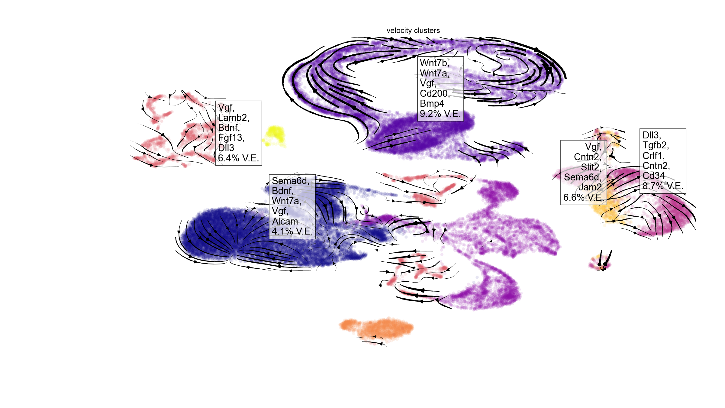
We can visualize the top ranked ligands at a glance with the function
en.plot_velocity_ligands_python(). By default, the function
only visualizes results with positive variance explained, with the
assumption that negative variance explained denotes poor model
accuracy.
en.plot_velocity_ligands_python(adata_result,
                                cell_palette="plasma",
                                velocity_cluster_palette = "black",
                                color="velocity_clusters",
                                plot_output_path = "plot_result1.png")
Step-by-step analysis:
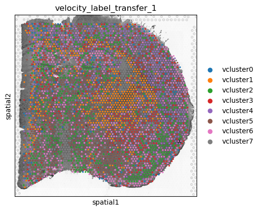
You may wish to perform label transfer separately from the ligand
inference. For example if you would like to manually inspect the label
transfer result before continuing. In this case, you might want to use
the following workflow. This consists of running
en.velocity_label_transfer(), viewing the labels on spatial
data, and inputting them into
en.get_velocity_ligands_spatial(). Make sure to specify
tangram_result_column = to prevent redundant analysis.
adata_st_transfer = en.velocity_label_transfer(adata,
                                               adata_st,
                                               plot="label_transfer_plot.png",
                                               organism="mouse",
                                               tangram_result_column = "velocity_label_transfer",
                                              velocity_cluster_key="velocity_clusters")

sc.pl.spatial(adata_st_transfer,
              color="velocity_label_transfer",
              save = "plot_labels.png")
Here, we are happy with these transferred velocity clusters. You can
now feed these labels back into
en.get_velocity_ligands_spatial(). Make sure to specify
tangram_result_column = and adata_st = to
prevent redundant analysis.
adata_result = en.get_velocity_ligands_spatial(adata,
                                               adata_st = adata_st_transfer,
                                               tangram_result_column = "velocity_label_transfer",
                                               ligand_target_matrix = ligand_target_matrix,
                                               velocity_cluster_key = "velocity_clusters",
                                               plot_output_path = "plot_result2.png")
Analysis on Cell clusters instead of Velocity clusters:
You may wish to run Entrain on your manually annotated populations rather than the velocity clusters that we generated here. We do not generally recommend this, because velocities do not always correlate exactly to cell annotations. However, there are situations where this may be useful e.g. analysis on rare cell populations that do not correlate with velocity clusters, or analysis on a single cell type of interest.
annotation_key = "broadlabel"
adata = en.recover_dynamics_clusters(adata,
                                     n_jobs = 10,
                                     cluster_key = annotation_key,
                                     return_adata = True)

adata_result=en.get_velocity_ligands_spatial(adata,
                                             adata_st,
                                             organism="mouse",
                                             velocity_cluster_key = annotation_key,
                                             ligand_target_matrix=ligand_target_matrix)

en.plot_velocity_ligands_python(adata_result,
                                cell_palette="Set1",
                                velocity_cluster_palette = "black",
                                color = annotation_key,
                                plot_output_path = "plot_result3.png")