Entrain ligand-velocity analysis • entrain

Entrain ligand-velocity analysis from an Anndata object.

This document outlines a basic Entrain analysis starting from an scverse anndata object with pre-calculated velocities. By the end of this document, you will identify ligands that are driving the velocities in your data.

Prior assumptions: Entrain-Velocity Analysis requires the following:

Single-Cell RNA data on a dataset of cells differentiating as well as data on their microenvironmental niche. The niche can be contained in a separate dataset (e.g., if you have sequenced in a separate capture) or in the same dataset as the differentiating cells.
A .h5ad object produced by scvelo that contains robust velocity data. Please ensure that your biology you are interested in is conducive to producing trustworthy velocities..
You have (some) idea of which cell clusters comprise the ‘niche’, or ligand-expressing cells, in your dataset.

library("Seurat"); library("SeuratWrappers");library("reticulate"); library("dplyr"); library("circlize");
library("entrain")

Pre-processing and loading required data.

Conda setup.

Because RNA velocity is natively done in python, this workflow involves calling python scripts from R to process the anndata object. The interfacing between python and R is handled by the package reticulate. We recommend using conda to setup a python environment that contains the required packages for velocity analysis.

reticulate::conda_create("r-reticulate-entrain")
reticulate::conda_install("r-reticulate-entrain", packages = c("scanpy", "leidenalg", "python-igraph", "adjustText", "loompy"), channel="conda-forge")
reticulate::conda_install("r-reticulate-entrain", packages = "scvelo", pip=TRUE)
reticulate::use_condaenv("r-reticulate-entrain")

Loading in required data

We will download a developing mouse brain atlas dataset at gestation day 10/11. This dataset contains both RNA expression and RNA velocities needed for our analysis. The following code block downloads the .gz file, decompresses it, and converts it into a Seurat object for analysis.

library("SeuratDisk")
options(timeout=3600)
h5ad_path <- "Manno_E10_E11.h5ad"
download.file("https://zenodo.org/record/7874401/files/Manno_E10_E11.h5ad.gz", "Manno_E10_E11.h5ad.gz")
system("gunzip Manno_E10_E11.h5ad.gz")
Convert("Manno_E10_E11.h5ad", dest = "h5seurat", overwrite = FALSE, verbose = TRUE)
obj <- LoadH5Seurat("Manno_E10_E11.h5seurat", assays="RNA")

Entrain relies on the NicheNet database of ligand-receptor-gene networks for the prior knowledge needed to make conclusions about environmentally-influenced trajectories. The genes here have been pre-converted from the original human genes to mouse orthologs.

lr_network_mm <- readRDS(url("https://zenodo.org/record/7874401/files/lr_network_mm.rds")) #
ligand_target_matrix_mm <- readRDS(url("https://zenodo.org/record/7874401/files/ligand_target_matrix_mm.rds"))

Data at a glance

The data consists of cells in the developing mouse brain at day 10 after gestation. This comprises a population of neuroblasts rapidly differentiating to neurons (our cells we are going to analyse), as well as their complex microenvironment made up of cells from the endoderm, mesoderm, fibroblastic, blood, and immune compartments.

n_clusters <- obj@meta.data$Class %>% unique() %>% length()
cols = Seurat::DiscretePalette(n = n_clusters, palette = "alphabet2")
DimPlot(obj, group.by = "Class", cols=cols)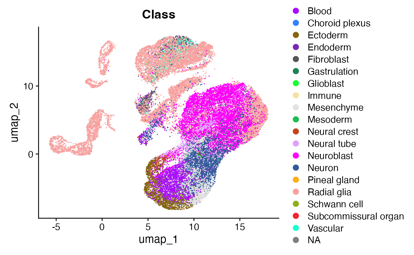

Run Entrain from a velocity anndata object.

Entrain fully integrates the scvelo package for velocity analysis. Below are the main steps:

Clustering Velocities

First, cluster velocities into groups of similar velocity dynamics. The resultant velocity clusters (or vclusters) are a separate entity from the usual cell annotation clusters. Cells of the same celltype cluster may not necessarily be in the same velocity cluster.

adata <- entrain_cluster_velocities(h5ad_path, resolution=0.1)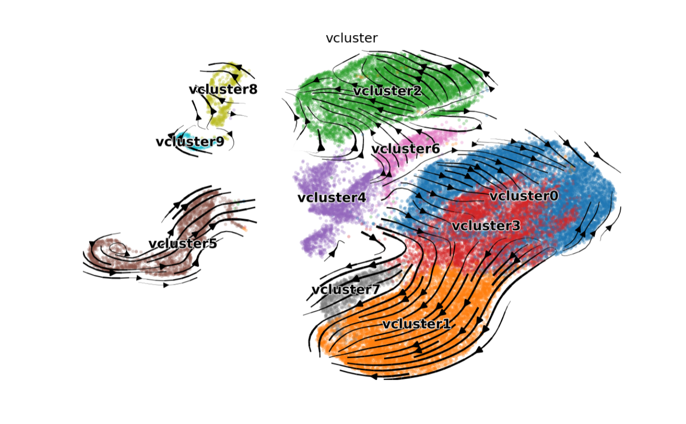

We can see that the velocity clusters roughly, but not exactly, correspond to cell type clusters, indicating that velocities are moderately correlated with cell type.

Fitting Ligands to Velocities

The fitting is encapsulated in the single function entrain_velocity(), shown below. This function firstly runs scvelo.tl.recover_dynamics() to rank genes based on their fit-likelihoods, a measure of a gene’s fit to the ordinary differential equation models that underlie RNA velocity derivation. Higher values denote more confidence in the velocity. Next, it runs Entrain analysis on the velocity likelihoods on a cluster-by-cluster basis.

We will also save the resulting .h5ad object for plotting our results afterwards.

sender_cluster_names <- c("Blood", "Fibroblast", "Immune", "Mesoderm")
Idents(obj) <- "Class"
save_adata =  "../../entrain_vignette_data/manno_entrain_result.h5ad"
obj_v <- entrain_velocity(receiver_obj = obj,
                          adata = adata,
                          save_adata = save_adata,
                          sender_cluster_key = "Class",
                          sender_clusters = sender_cluster_names,
                          lr_network = lr_network_mm,
                          num_top_genes = NULL,
                          ligand_target_matrix = ligand_target_matrix_mm)

Note that as of July 2023, there is an existing bug in scvelo.tl.recover_dynamics(). Using `numpy version 1.23.5 may fix the problem. Also see #1058.

Visualizing results

At a glance

We can visualize the top ranked ligands at a glance with the function plot_velocity_ligands(). By default, the function only visualizes results with positive variance explained, with the assumption that negative variance explained denotes poor model accuracy.

plot_velocity_ligands(adata=save_adata,
                      plot_output_path = "manno_entrain.png")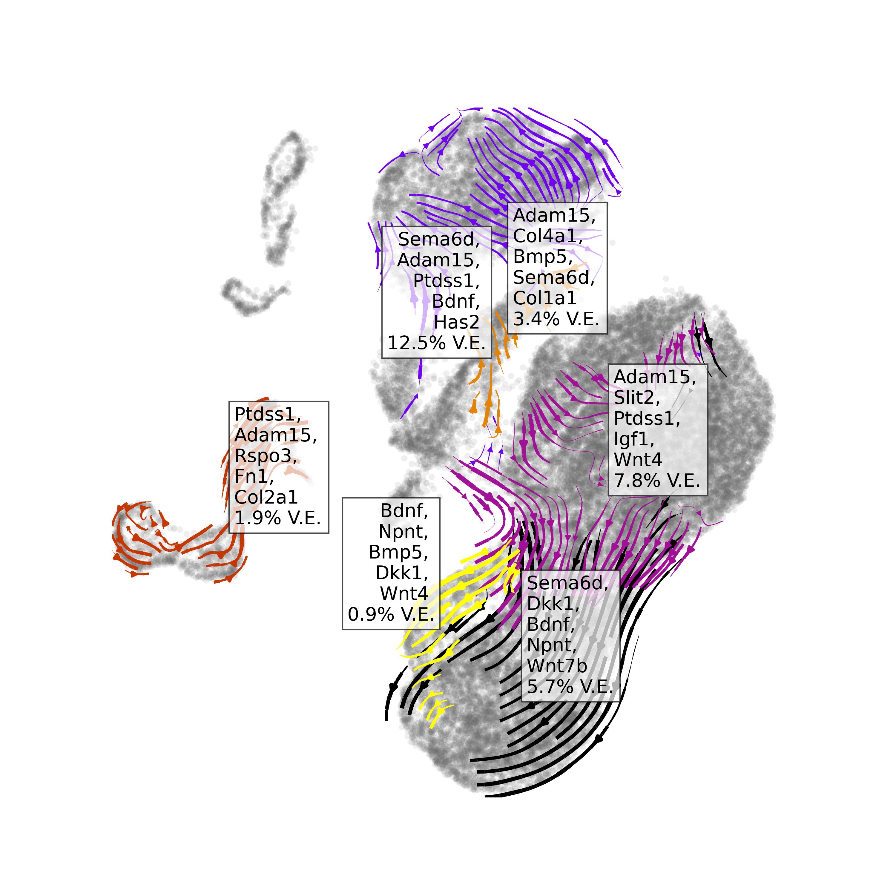

This suggests a number of ligands responsible for neurogenic differentiation processes. These are well-established in literature as key drivers for cell differentiation.

In detail

Entrain-Velocity provides detailed plotting functions for visualizing extracellular and intracellular regulation predicted to be driving the observed velocities.

Sender Cell Visualization

Visualization of cells that express the ligands found in our analysis. Cells are coloured based on mean expression of the top_n_ligands predicted to be driving velocities in the velocity cluster.

vclusters_to_plot <- c("vcluster0", "vcluster1", "vcluster2", "vcluster3")
save_adata =  "../../entrain_vignette_data/manno_entrain_result.h5ad"
plot_sender_influence_velocity(adata= save_adata,
                                   velocity_clusters = vclusters_to_plot,
                                   title = "velocity_sender_influences.png")

#### Visualizing ligand importances Visualization of ligands and their relative importances, or contribution, towards each vcluster.

g<-velocity_ligand_importance_heatmap(obj_v,
                                     n_top_ligands=5) +
    ggplot2::scale_fill_viridis_c(option="inferno")
g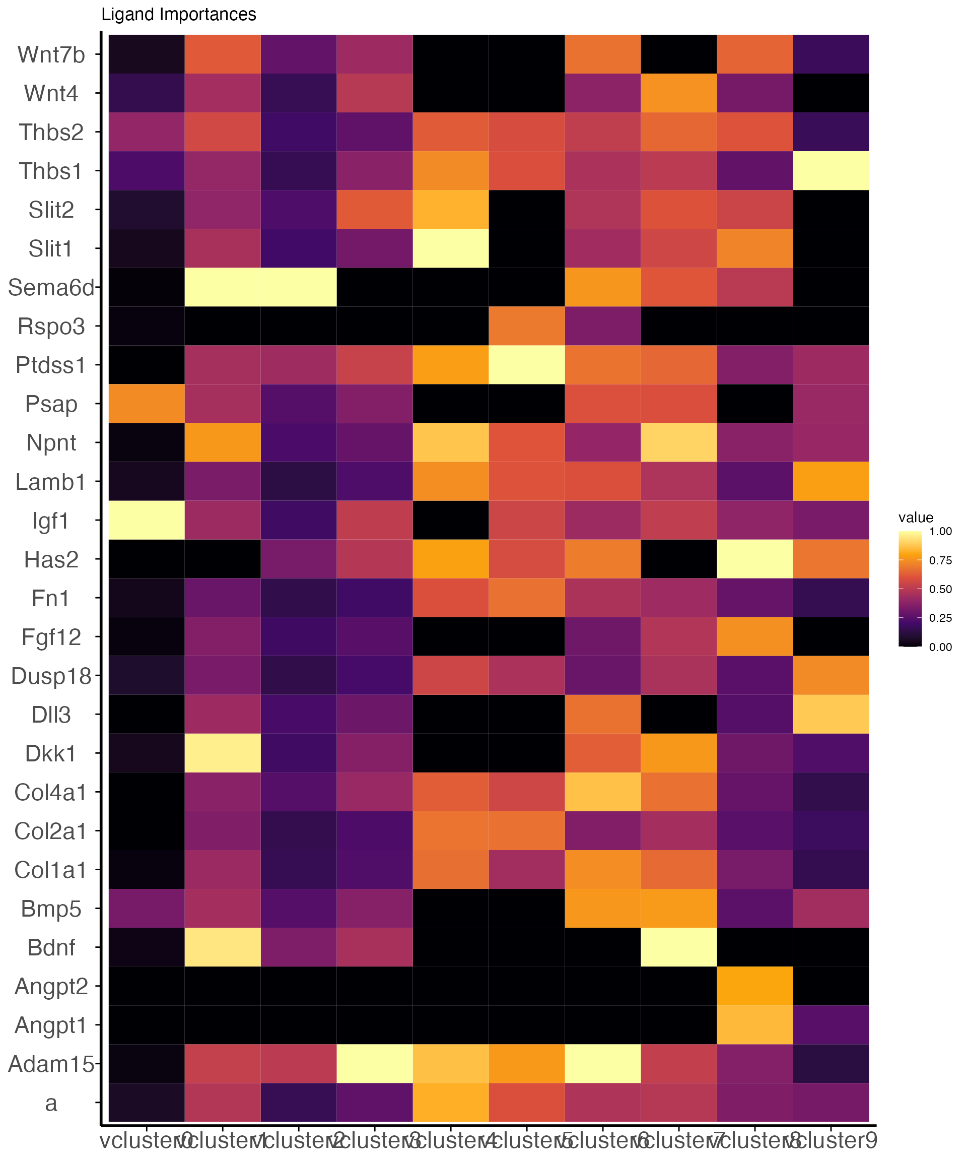

Visualizing high velocity likelihood genes

Commonly, a small proportion of the total genes contribute the majority of the observed RNA velocity dynamics. You may wish to visualize these genes by plotting the top likelihood genes as a sanity check to confirm that scvelo is appropriate for your biological system. These genes are the ones found by scvelo to most robustly fit the underlying theoretical model. The function plot_velocity_likelihoods_heatmap() plots, as a heatmap, the n_top_genes ranked by velocity likelihood for each velocity cluster.

g<-plot_velocity_likelihoods_heatmap(obj_v,
                                     n_top_genes=5)
g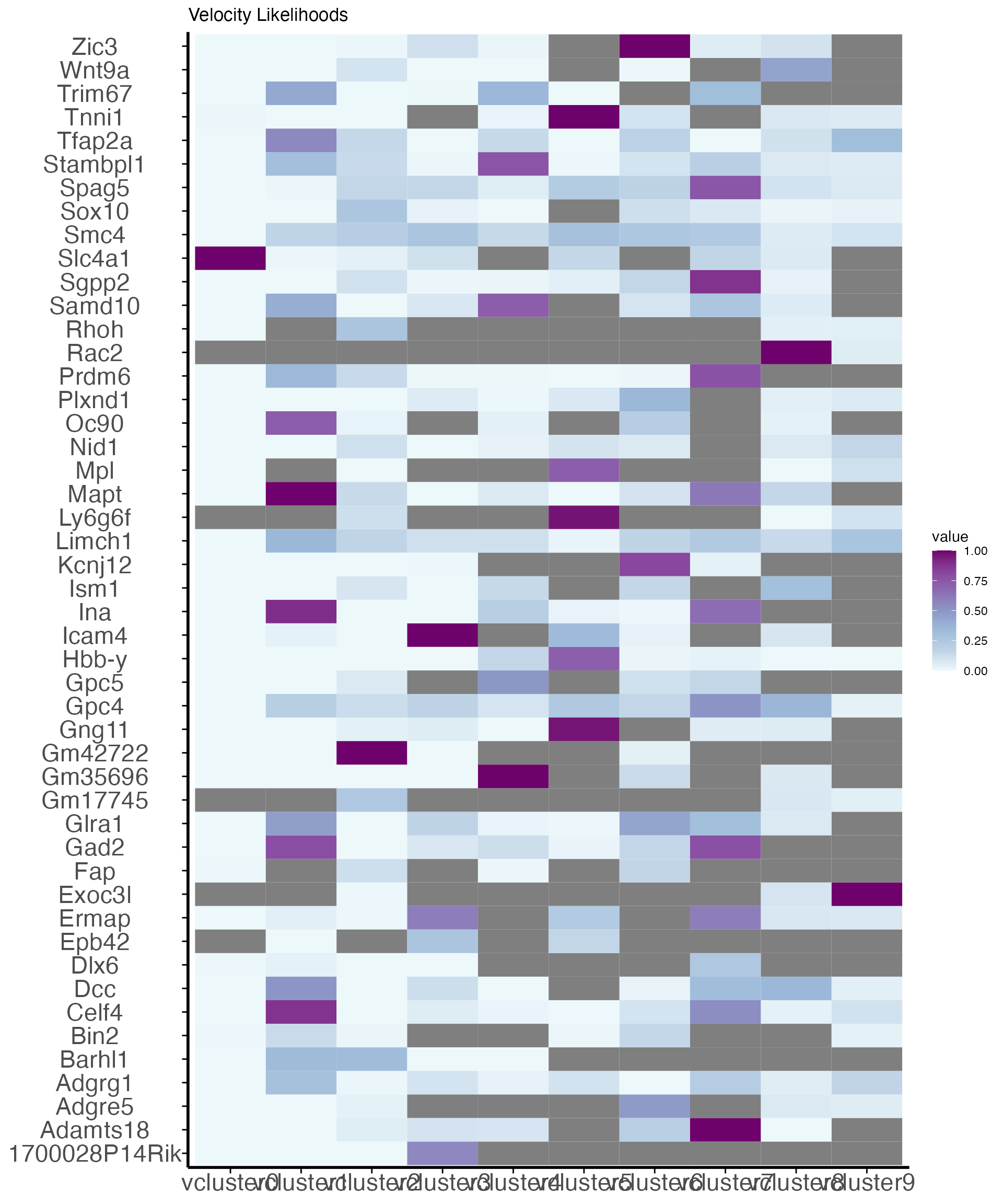

Visualizing intracellular regulation downstream of the ligand-receptor pair.

The function plot_velocity_ligand_targets extracts regulatory information from NicheNetR to visualize the predicted regulatory linkages between the n_top_ligands and the n_top_targets high velocity likelihood genes.

g<-plot_velocity_ligand_targets(obj_v,
                                velocity_cluster="vcluster1",
                                n_top_ligands=10L,
                                ligand_target_matrix=ligand_target_matrix_mm)
g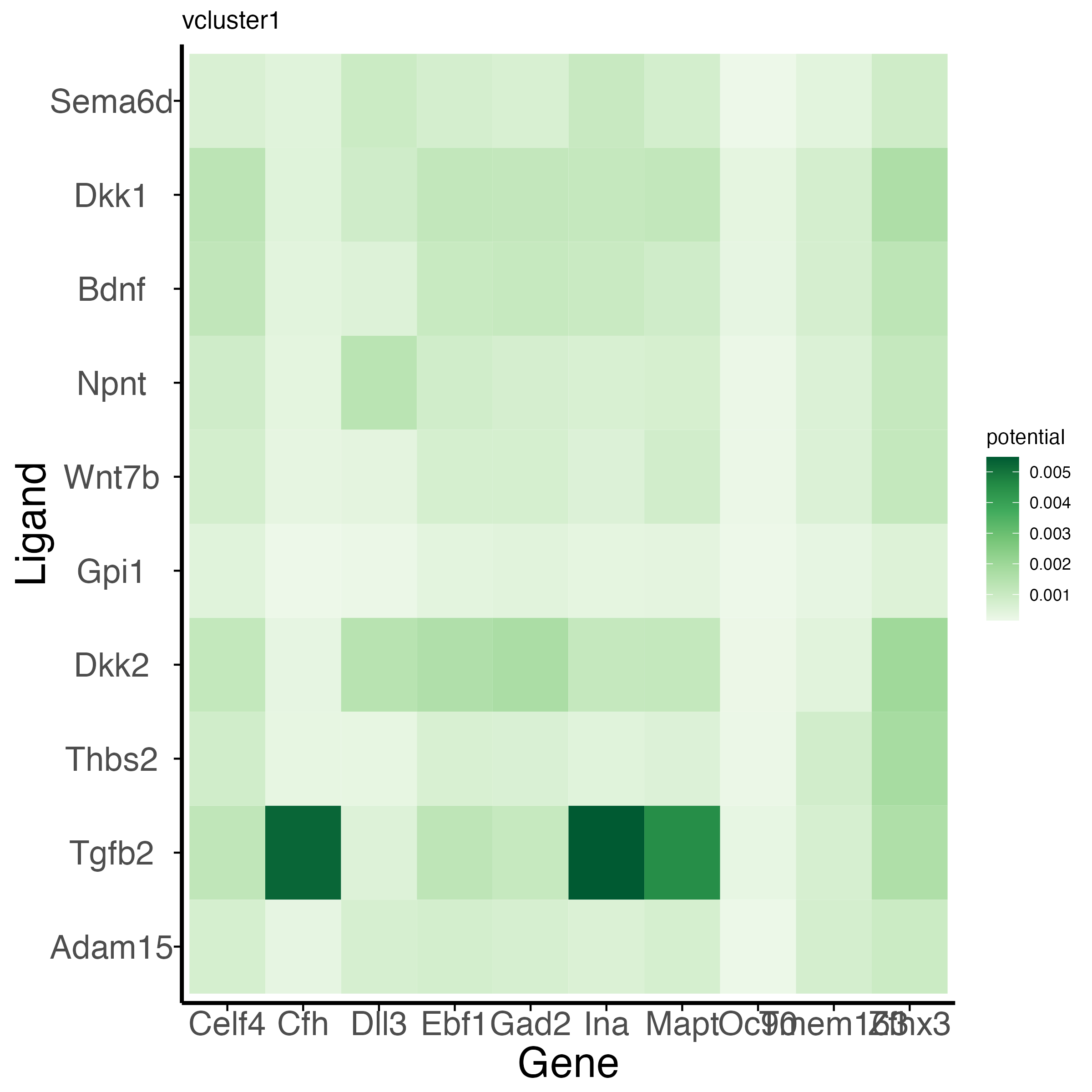

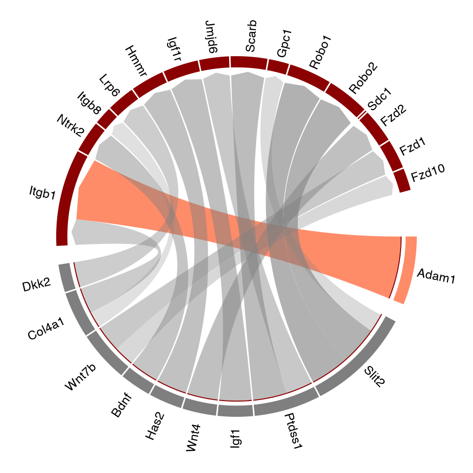
Visualization with a circos plot

Circos plots are a popular format for visualizing connections between ligand receptor pairs. We recreate this method with the function draw_entrain_circos(), making sure to feed it NicheNet’s weighted database: weighted_networks.

weighted_networks <- readRDS(url("https://zenodo.org/record/7874401/files/weighted_networks_mm.rds"))

draw_entrain_circos(obj = obj_v,
                    vcluster= "vcluster3",
                    lr_network = lr_network_mm,
                    weighted_networks = weighted_networks)

## Warning in RColorBrewer::brewer.pal(length(ligand_types), palette): minimal value for n is 3, returning requested palette with 3 different levels